Chapter 5 Classification Models for Customer Segmentation

5.1 Fundamentals of Customer Segmentation

Customer segmentation is an essential marketing strategy that categorizes a company’s customers into distinct groups with common characteristics, behaviors, or preferences. This approach allows businesses to tailor their marketing strategies, product offerings, and customer interactions to meet the specific needs and expectations of each segment. When executed effectively, customer segmentation enhances resource allocation, boosts customer satisfaction and loyalty, and drives growth and profitability.

Traditionally, segmentation has relied on demographic, geographic, and psychographic criteria. Demographics analyze age, gender, income, education, and occupation; geography sorts customers by their physical locations, such as countries, regions, or cities; and psychographics assess personality traits, values, and lifestyles. While these traditional methods have proven effective, they may not capture the complete picture in today’s data-rich environment.

The rise of big data and analytics has positioned machine learning as a transformative tool for customer segmentation. Machine learning algorithms can sift through vast datasets, identifying intricate patterns and insights beyond the reach of traditional segmentation methods. The advantages of machine learning in this context include:

1. Enhanced Precision: Machine learning reveals complex relationships within customer data, offering more accurate and nuanced segmentation.

2. Scalability: Automated processes efficiently manage significant data volumes, evolving with the customer base and ensuring segmentation models remain current.

3. Dynamic Updates: Machine learning adapts to ongoing data flow, allowing for real-time refinement of customer segments.

4. Predictive Insights: Beyond current trends, machine learning anticipates future customer behaviors and preferences, facilitating forward-looking marketing strategies.

5. Comprehensive Data Integration: By analyzing diverse data sources, including transaction records, digital footprints, and customer feedback, machine learning provides a holistic customer view.

6. Personalization: Tailored experiences are developed through deep insights into customer segments and individual preferences, fostering enhanced engagement and loyalty.

Subsequent sections will explore popular machine learning techniques for customer segmentation, including K-Means clustering, hierarchical clustering, Gaussian Mixture Models (GMM), Self-Organizing Maps (SOM), and DBSCAN. We will also guide you through constructing K-Means and LLM+K-Means models with practical datasets for advanced marketing analytics.

5.2 Popular Models for Customer Segmentation

5.2.1 K-Means Clustering

K-Means clustering, a dominant unsupervised machine learning technique, efficiently segments customers by partitioning observations into k clusters, based on the nearest mean (centroid). The objective is to minimize the within-cluster sum of squares (WCSS), essentially the squared distances between data points and their respective centroids.

Advantages:

• Simplicity: Its straightforward nature makes K-Means accessible for a broad audience.

• Efficiency: Capable of managing large datasets, it’s well-suited for extensive customer segmentation tasks.

• Scalability: Adapts well to high-dimensional data, enhanced by appropriate initialization and distance measures.

Limitations:

• Initialization Sensitivity: Initial centroid placement can significantly affect outcomes, potentially leading to less optimal clusterings.

• Spherical Cluster Assumption: Assumes clusters are spherical and equally sized, which may not align with real customer data distributions.

• Cluster Number Specification: Requires pre-determined cluster numbers (k), which can be challenging without prior data insights.

• Outlier Sensitivity: Outliers can skew centroids, impacting clustering accuracy.

5.2.2 Hierarchical Clustering

Hierarchical clustering offers a nuanced approach to customer segmentation by building a dendrogram, a tree-like structure that displays observation groupings at various granularity levels. It diverges from K-Means by not necessitating a predefined cluster count and can be executed in two main forms:

1. Agglomerative (bottom-up): Begins with each observation as an individual cluster, progressively merging the nearest pairs until a singular cluster remains. Common linkage criteria include:

   • Single linkage: Minimum distance between cluster observations.

   • Complete linkage: Maximum distance between cluster observations.

   • Average linkage: Average distance across all observation pairs within two clusters.

   • Ward’s linkage: Merge based on the smallest increase in total within-cluster variance.

2. Divisive (top-down): Starts with all observations in one cluster, systematically dividing into smaller clusters. Due to its higher computational demand, it’s less commonly applied.

Dendrogram Insights: The dendrogram visualizes the hierarchical clustering outcome, showing the sequential merging or splitting of clusters. It allows for determining the optimal cluster count by cutting the dendrogram at a desired distance or height.

Advantages:

• No Cluster Count Pre-specification: It doesn’t require an upfront cluster number.

• Granularity Flexibility: Users can select segmentation granularity by adjusting the dendrogram cut height.

• Non-spherical Cluster Handling: Effectively identifies clusters of varied shapes and sizes, offering a realistic segmentation.

Limitations:

• Computational Intensity: Higher computational complexity than K-Means, particularly for larger datasets.

• Noise and Outlier Sensitivity: Especially with single linkage, noise and outliers can merge unrelated clusters.

• Irreversible Merging/Splitting: Decisions are final, potentially leading to suboptimal outcomes.

Applying hierarchical clustering necessitates careful data preprocessing, selecting a suitable linkage criterion, and thorough dendrogram analysis to align segmentation with business goals.

5.2.3 Gaussian Mixture Models (GMM)

Gaussian Mixture Models (GMM) employ a probabilistic technique for clustering, positing that data originates from several Gaussian distributions. Each cluster is characterized by its mean, covariance matrix, and mixing coefficient, with the objective of GMM being to estimate these parameters and assign data points to the most probable cluster based on posterior probabilities.

Expectation-Maximization (EM) Algorithm for GMM: The EM algorithm iteratively refines the GMM parameters through two phases:

1. Expectation (E-step): Calculate the posterior probabilities for each data point’s cluster membership using current parameter estimates.

2. Maximization (M-step): Update the model parameters (means, covariances, and mixing coefficients) to maximize the expected log-likelihood of the observed data, leveraging the posterior probabilities from the E-step.

This cycle continues until the parameters converge or a predefined number of iterations is achieved.

Advantages:

• Soft Clustering: Offers probabilistic cluster assignments, enabling nuanced and potentially overlapping segments.

• Flexible Cluster Shapes: Capable of modeling clusters of different sizes and shapes due to the varied covariance structures.

• Probabilistic Interpretation: Provides a measure of cluster membership uncertainty, useful for evaluating segmentation reliability.

Limitations:

• Gaussian Assumption: Assumes data within each cluster follows a Gaussian distribution, which may not align with all real-world scenarios.

• Initialization Sensitivity: Outcomes can vary based on the initial parameter values, potentially leading to different local optima.

• Computational Demand: High, especially with large datasets and numerous clusters, due to the complexity of the EM algorithm.

5.2.4 Self-Organizing Maps (SOM)

Self-Organizing Maps (SOM), or Kohonen maps, are a type of unsupervised neural network for clustering and visualizing high-dimensional data in a lower-dimensional (typically 2D) space, preserving the topological properties of the original data. This mapping aims to place similar data points close on the 2D grid, facilitating cluster analysis.

SOM Algorithm:

1. Initialize neuron weights in the 2D grid randomly.

2. For each input, identify the best matching unit (BMU) — the neuron whose weight vector is closest to the input.

3. Adjust the weights of the BMU and its neighbors to better match the input, influenced by a learning rate and a neighborhood function.

4. Iterate through steps 2 and 3 until the system stabilizes or completes a fixed number of iterations.

Visualization and Interpretation:

• U-matrix: Highlights distances between neurons to delineate clusters and outliers.

• Component Planes: Depicts how individual features distribute across the grid, revealing patterns and correlations.

• SOM Grid Clustering: Further clustering (e.g., with K-Means) on the SOM output can refine segmentation.

Advantages:

• Dimensionality Reduction: Offers a manageable, visual representation of complex datasets.

• Topology Preservation: Ensures that similar segments are mapped closely, aiding interpretability.

• Missing Value Tolerance: Can train with incomplete data sets by disregarding missing values.

Limitations:

• Indirect Clustering: Does not explicitly define clusters, necessitating further analysis.

• Grid Size Sensitivity: The choice of grid dimensions can significantly impact performance and outcomes.

• Interpretation Challenges: Complex data traits or a high feature count can complicate results analysis.

5.2.5 DBSCAN (Density-Based Spatial Clustering of Applications with Noise)

DBSCAN excels in identifying clusters of any shape while managing noise and outliers, without pre-specifying a cluster count. It distinguishes clusters as dense regions, separated by less dense areas.

DBSCAN Overview: Data points are classified as:

1. Core Points: Have a minimum number of neighbors within a specified radius (epsilon).

2. Border Points: Near a core point but don’t meet the core point criteria themselves.

3. Noise Points: Neither core nor border points.

Starting from a core point, DBSCAN expands clusters by incorporating neighboring core and border points, proceeding to the next unvisited core point until all are processed.

Advantages:

• Arbitrary Shape Clustering: Identifies non-spherical clusters, fitting various data distributions.

• Outlier Resistance: Effectively segregates noise and outliers from main clusters.

• No Preset Clusters: Eliminates the need to define the number of clusters upfront.

Parameter Selection (epsilon and min_samples):

• Epsilon (ε): Dictates the maximum distance for points to be considered as in the same cluster. Varying epsilon affects cluster size and count.

• Min_samples: Determines the density threshold for core points, influencing cluster robustness and noise sensitivity.

Selecting these parameters is critical and can be aided by techniques like the k-distance plot to identify an appropriate epsilon.

Implementing DBSCAN with Scikit-learn involves data preprocessing, instantiating a DBSCAN object with chosen parameters, fitting it to data, and analyzing the results.

Interpreting DBSCAN: The output categorizes points into clusters or as noise (-1). Visualizing these assignments helps understand the segmentation, which can be further analyzed through feature examination and cluster quality metrics.

DBSCAN’s effectiveness in customer segmentation hinges on careful parameter choice, informed by data properties and segmentation objectives. Its ability to manage complex cluster shapes and noise makes it a versatile tool for exploratory segmentation tasks.

5.3 K-Means Clustering Model Development on Kaggle’s Banking Dataset

This section outlines the process of developing a K-Means clustering classification model for customer segmentation using the public Banking Dataset - Marketing Targets available on Kaggle. This dataset includes bank customers’ demographic details, financial attributes, and responses to marketing campaigns. We will conduct exploratory data analysis (EDA), preprocess the data, and utilize the Scikit-learn library in Python to implement K-Means clustering.

5.3.1 Dataset Description

Banking Dataset - Marketing Targets Overview: The Banking Dataset - Marketing Targets, accessible on Kaggle, offers insights into bank customers’ profiles and behaviors. It comprises 45,211 records with 17 features, including:

• age: Customer’s age

• job: Customer’s job type (e.g., management, technician, entrepreneur)

• marital: Marital status (married, single, divorced)

• education: Education level (e.g., primary, secondary, tertiary)

• default: Credit default status (yes, no)

• balance: Average yearly balance

• housing: Housing loan status (yes, no)

• loan: Personal loan status (yes, no)

• contact: Contact method (e.g., cellular, telephone)

• day & month: Last contact day and month

• duration: Last contact duration (seconds)

• campaign: Contacts during the current campaign

• pday & previous: Days since last contact and previous contact count

• poutcome: Previous campaign outcome (e.g., success, failure)

• y: response of subscription to bank’s term deposit (yes, no)

import pandas as pd 

df_train = pd.read_csv("data\Chapter5_train.csv", sep=";", header=0)
df_test = pd.read_csv("data\Chapter5_test.csv", sep=";", header=0)

print(df_train.shape)
print(df_test.shape)

(45211, 17)
(4521, 17)

df_train.head()

	age	job	marital	education	default	balance	housing	loan	contact	day	month	duration	campaign	pdays	previous	poutcome	y
0	58	management	married	tertiary	no	2143	yes	no	unknown	5	may	261	1	-1	0	unknown	no
1	44	technician	single	secondary	no	29	yes	no	unknown	5	may	151	1	-1	0	unknown	no
2	33	entrepreneur	married	secondary	no	2	yes	yes	unknown	5	may	76	1	-1	0	unknown	no
3	47	blue-collar	married	unknown	no	1506	yes	no	unknown	5	may	92	1	-1	0	unknown	no
4	33	unknown	single	unknown	no	1	no	no	unknown	5	may	198	1	-1	0	unknown	no

5.3.2 EDA and Data Preprocessing:

Key preprocessing steps include:

1. Missing Values: Identify and address missing values through removal or imputation.

2. Categorical Variables: Convert categories into numerical forms via one-hot or label encoding.

3. Feature Scaling: Normalize numerical features to ensure equal impact on clustering.

4. Feature Analysis: Assess distributions and correlations among features using visual tools.

5. Outliers: Detect and address outliers with methods like Z-score or IQR.

We will use Python package ‘Sweetviz’ to generate an EDA report automatically. By setting the target feature as “y”, we can understand better the response (subscription) rate pattern by feature segments.

# convert y to 0 and 1: 0 for "no" and 1 for "yes"
df_train["y"] = df_train["y"].apply(lambda x: 0 if x == "no" else 1)
df_test["y"] = df_test["y"].apply(lambda x: 0 if x == "no" else 1)

# use sweetviz to generate a report
import sweetviz as sv
report = sv.analyze(df_train, target_feat = "y")
report.show_html("results\chapter5_eda_report.html")

For simplicity, we will use one-hot encoding method to convert categorical variables to numerical features.

# use one-hot encoding to convert categorical variables to numerical
df_train_encoded = pd.get_dummies(df_train, drop_first=True)
df_test_encoded = pd.get_dummies(df_test, drop_first=True)
df_train_encoded.head()

	age	balance	day	duration	campaign	pdays	previous	y	job_blue-collar	job_entrepreneur	...	month_jul	month_jun	month_mar	month_may	month_nov	month_oct	month_sep	poutcome_other	poutcome_success	poutcome_unknown
0	58	2143	5	261	1	-1	0	0	0	0	...	0	0	0	1	0	0	0	0	0	1
1	44	29	5	151	1	-1	0	0	0	0	...	0	0	0	1	0	0	0	0	0	1
2	33	2	5	76	1	-1	0	0	0	1	...	0	0	0	1	0	0	0	0	0	1
3	47	1506	5	92	1	-1	0	0	1	0	...	0	0	0	1	0	0	0	0	0	1
4	33	1	5	198	1	-1	0	0	0	0	...	0	0	0	1	0	0	0	0	0	1

5 rows × 43 columns

# feature scaling min-max   
from sklearn.preprocessing import MinMaxScaler
scaler = MinMaxScaler()

X_train = df_train_encoded.drop("y", axis=1)
X_train_scaled = scaler.fit_transform(X_train)
y_train = df_train_encoded["y"]

X_test = df_test_encoded.drop("y", axis=1)
X_test_scaled = scaler.transform(X_test)
y_test = df_test_encoded["y"]

# convert the scaled data to a dataframe
df_X_train_scaled = pd.DataFrame(X_train_scaled, columns=X_train.columns)
df_X_test_scaled = pd.DataFrame(X_test_scaled, columns=X_test.columns)
df_train_encoded_scaled = pd.concat([df_X_train_scaled, y_train], axis=1)
df_test_encoded_scaled = pd.concat([df_X_test_scaled, y_test], axis=1)

5.3.3 Implementing K-Means Clustering

5.3.3.1 Selecting the Optimal Number of Clusters (Elbow Method)

We will use the Elbow method to determine the ideal cluster count (k) by plotting the within-cluster sum of squares (WCSS) against the number of clusters and identifying the “elbow” point.

from sklearn.cluster import KMeans
from yellowbrick.cluster import KElbowVisualizer

model = KMeans(init='k-means++')
visualizer = KElbowVisualizer(model, k=(4,12),metric="distortion") 
visualizer.fit(X_train_scaled)
visualizer.show()

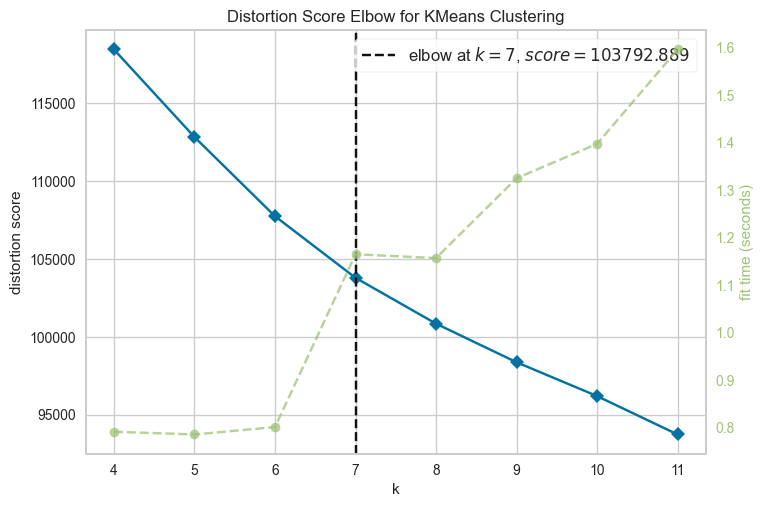
<AxesSubplot:title={'center':'Distortion Score Elbow for KMeans Clustering'}, xlabel='k', ylabel='distortion score'>

5.3.3.2 Applying K-Means Clustering

The generated figure indicates that the optimal cluster number is seven. By specifying n_clusters=7, we fit the KMeans clustering model with the optimal number of clusters and assign the cluster number to each individual customer.

from sklearn.cluster import KMeans

kmeans = KMeans(n_clusters=7, init='k-means++', random_state=42)
kmeans.fit(X_train_scaled)
df_train_encoded_scaled["Cluster"] = kmeans.labels_

5.3.3.4 Evaluating the performance of a K-means clustering model

K-Means clustering model involves determining the effectiveness of the data partitioning into distinct clusters. Unlike supervised learning models, which utilize accuracy, precision, and recall for evaluation, unsupervised clustering models require alternative approaches due to the absence of predefined labels. Here are several methods used to evaluate K-means clustering models:

Inertia or Within-Cluster Sum of Squares (WCSS): Inertia quantifies the compactness of the clusters, calculating the sum of squared distances of each data point to its nearest centroid. The objective is to minimize inertia, indicating dense and well-separated clusters. However, reducing the cluster count to 1 results in zero inertia, presenting a trade-off. An inertia plot against the number of clusters (elbow method) helps identify the optimal cluster count by locating the “elbow point,” where the rate of decrease in inertia markedly shifts.

Silhouette Score: The Silhouette Score assesses how similar an object is to its cluster (cohesion) versus other clusters (separation). Scores range from -1 to 1, where higher values indicate strong matching within the cluster and poor matching to neighboring clusters. Predominantly high values suggest a suitable clustering configuration.

Davies-Bouldin Index: The Davies-Bouldin Index (DBI) evaluates clustering quality based on the ratio of within-cluster to between-cluster distances. Lower DBI values indicate better clustering by favoring compact and well-separated clusters.

Calinski-Harabasz Index: Also known as the Variance Ratio Criterion, this index evaluates clustering by comparing the ratio of between-cluster dispersion to within-cluster dispersion across all clusters. Higher values signify better clustering performance, reflecting dense and distinct clusters.

All these metrics can be obtained through sklearn Python package which makes the metrics calculation much easier.

from sklearn.metrics import silhouette_score, davies_bouldin_score, calinski_harabasz_score

def evaluate_clustering(X, labels, model):
    """
    Evaluate clustering performance using various metrics.
    
    Parameters:
    - X: The dataset used for clustering (features).
    - labels: The labels predicted by the clustering model.
    - model: The fitted clustering model (e.g., KMeans instance).
    
    Returns:
    A dictionary containing the Inertia, Silhouette Score, Davies-Bouldin Index, and Calinski-Harabasz Index.
    """
    metrics = {}
    
    # Inertia
    metrics['Inertia'] = model.inertia_
    
    # Silhouette Score
    metrics['Silhouette Score'] = silhouette_score(X, labels, sample_size=5000)
    
    # Davies-Bouldin Index
    metrics['Davies-Bouldin Index'] = davies_bouldin_score(X, labels)
    
    # Calinski-Harabasz Index
    metrics['Calinski-Harabasz Index'] = calinski_harabasz_score(X, labels)
    
    return metrics

metrics = evaluate_clustering(X_train_scaled, kmeans.labels_, kmeans)
print(metrics)

{'Inertia': 103927.74320527555, 'Silhouette Score': 0.12321804390553139, 'Davies-Bouldin Index': 2.371944407695371, 'Calinski-Harabasz Index': 3822.0899747713497}

5.3.4 Interprete the results

By calculating the mean values of each feature by Cluster, we can create the profile for each cluster.

# cluster profiling: mean values of each feature for each cluster
cluster_profile = df_train_encoded_scaled.groupby("Cluster").mean()
# write the cluster_profile to a csv file
cluster_profile.to_csv("results\chapter5_cluster_profile.csv")

After encoding and scaling the data frame, traditional methods of deriving explainable insights become challenging. However, leveraging Language Model prompts (LLM) simplifies the extraction of insights from cluster profiles. Through the LLM prompt, we can not only catalog the features of each cluster but also provide tailored marketing strategy recommendations for each segment.

Cluster	Age Group	Average Balance	Campaign Interaction Timing	Dominant Job Roles	Contact Months	Campaign Outcome (Success Rate)	Marketing Strategy Recommendations
0	Mixed, younger to middle-age	Moderate	Middle of the month, moderate duration	Diverse, entrepreneurs	Throughout the year, peak in May and November	Moderate	Diversify messaging to appeal to a wide age range; emphasize entrepreneurial spirit.
1	Younger to middle-age	Slightly lower	Predominantly in May, fewer follow-ups	Strongly blue-collar	May	Lower	Focus on value and practical benefits; leverage direct, clear communication.
2	Similar to 0 and 1, slightly older	Similar to 0 and 1	Almost exclusive in June	Blue-collar, entrepreneurs	June	Lower, minimal previous engagement	Intensify efforts in June with targeted offers; highlight opportunities for growth and investment.
3	Younger demographic	Comparable to others	End of the month, slightly longer interactions	Diverse, fewer blue-collar	Evenly distributed, preference for May and November	Higher	Utilize digital channels and social media; focus on innovation and tech-savviness.
4	Oldest	Similar to others	Later in the month, moderate interaction	Mix, less blue-collar	Varied, no specific peak month	Moderately high	Personalize communication; emphasize security, stability, and long-term benefits.
5	Youngest	Slightly lower	Middle of the month, slightly longer than average	Varied, significant blue-collar presence	High activity in May, but less exclusively	Moderately high	Craft youthful, energetic campaigns; focus on affordability and starting early on financial planning.
6	Younger to middle-age, slightly older than Cluster 5	Comparable to others	Later in the month, similar to Cluster 4	Strongly blue-collar	Less concentrated, notable absence in May	Lower	Adopt a hands-on approach with real-life examples; emphasize trustworthiness and reliability of services or products offered.

These marketing strategy recommendations are tailored to each cluster’s unique characteristics and campaign interaction patterns, aiming to enhance engagement and improve the success rate of future campaigns.

5.4 LLM+K-Means Clustering for Customer Segmentation

from sentence_transformers import SentenceTransformer

df_train.head()

	age	job	marital	education	default	balance	housing	loan	contact	day	month	duration	campaign	pdays	previous	poutcome	y
0	58	management	married	tertiary	no	2143	yes	no	unknown	5	may	261	1	-1	0	unknown	0
1	44	technician	single	secondary	no	29	yes	no	unknown	5	may	151	1	-1	0	unknown	0
2	33	entrepreneur	married	secondary	no	2	yes	yes	unknown	5	may	76	1	-1	0	unknown	0
3	47	blue-collar	married	unknown	no	1506	yes	no	unknown	5	may	92	1	-1	0	unknown	0
4	33	unknown	single	unknown	no	1	no	no	unknown	5	may	198	1	-1	0	unknown	0

def compile_text(x):
    text_list = [f"{col.capitalize()}: {x[col]}" for col in columns]
    text_string = ",\n".join(text_list)
    text = f'"""{text_string}"""'
    return text

df = df_train.head(5)
df 

	age	job	marital	education	default	balance	housing	loan	contact	day	month	duration	campaign	pdays	previous	poutcome	y	Cluster
0	58	management	married	tertiary	no	2143	yes	no	unknown	5	may	261	1	-1	0	unknown	0	2
1	44	technician	single	secondary	no	29	yes	no	unknown	5	may	151	1	-1	0	unknown	0	6
2	33	entrepreneur	married	secondary	no	2	yes	yes	unknown	5	may	76	1	-1	0	unknown	0	3
3	47	blue-collar	married	unknown	no	1506	yes	no	unknown	5	may	92	1	-1	0	unknown	0	0
4	33	unknown	single	unknown	no	1	no	no	unknown	5	may	198	1	-1	0	unknown	0	4

columns = df_train.drop(columns=['y']).columns
sentences = df_train.apply(compile_text, axis=1).tolist()
print(sentences[0])

"""Age: 58,
Job: management,
Marital: married,
Education: tertiary,
Default: no,
Balance: 2143,
Housing: yes,
Loan: no,
Contact: unknown,
Day: 5,
Month: may,
Duration: 261,
Campaign: 1,
Pdays: -1,
Previous: 0,
Poutcome: unknown,
Cluster: 2"""

model = SentenceTransformer(r"sentence-transformers/paraphrase-MiniLM-L6-v2")

from torch.utils.data import DataLoader

# Define a batch size
batch_size = 64

# Create a DataLoader
dataloader = DataLoader(sentences, batch_size=batch_size)

# Encode sentences in batches
output = []
for batch in dataloader:
    batch_output = model.encode(batch, show_progress_bar=True, normalize_embeddings=True)
    output.extend(batch_output)

df_embedding = pd.DataFrame(output)

df_embedding.to_csv("results\chapter5_embedding_train.csv")

When working with large dataframes, the embedding process may fail without optimization. The SentenceTransformer model, a transformer-based solution for text data, is inherently efficient. However, several strategies can further enhance your code’s efficiency:

Batch Processing: If your sentences list is very large, you might want to consider processing the sentences in batches. This can be done by splitting the sentences list into smaller lists and then encoding each smaller list separately. This can help to reduce memory usage.

GPU Acceleration: If you have a compatible GPU, you can use it to accelerate the encoding process. The SentenceTransformer model automatically uses the GPU if it is available. You can check if a GPU is available and set the device to GPU using PyTorch’s torch.cuda module.

Preprocessing: Depending on your specific use case, you might be able to make the encoding process more efficient by preprocessing your sentences. This could involve removing unnecessary words or characters, or converting all text to lowercase.

Parallel Processing: If you have a multi-core CPU, you can use parallel processing to encode multiple sentences at the same time. This can be done using Python’s multiprocessing module.

We have now generated embeddings for all features. Subsequently, we employ the Elbow method to determine the optimal number of clusters.

model_llm = KMeans(init='k-means++')
visualizer_llm = KElbowVisualizer(model_llm, k=(4,12),metric="distortion") 
visualizer_llm.fit(df_embedding)
visualizer_llm.show()

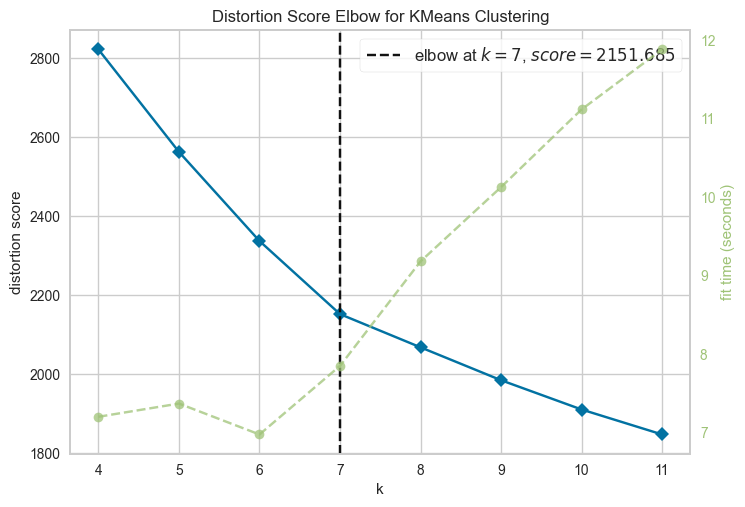
<AxesSubplot:title={'center':'Distortion Score Elbow for KMeans Clustering'}, xlabel='k', ylabel='distortion score'>

After identifying the optimal number of clusters, we continue to train a K-Means classifier on the embedding dataframe.

llm_kmeans = KMeans(n_clusters=7, init='k-means++', random_state=42)
llm_kmeans.fit(df_embedding)
df_train["Cluster"] = llm_kmeans.labels_

metrics_llm = evaluate_clustering(df_embedding, llm_kmeans.labels_, llm_kmeans)
print(metrics_llm)

{'Inertia': 2151.683837890625, 'Silhouette Score': 0.2150295, 'Davies-Bouldin Index': 1.6160626787772425, 'Calinski-Harabasz Index': 6742.381848334127}

Comparing four key performance metrics reveals a significant improvement in the LLM+K-Means classification model’s performance.

print(round(metrics_llm['Inertia'] / metrics['Inertia'], 3))
print(round(metrics_llm['Silhouette Score'] / metrics['Silhouette Score'], 3))
print(round(metrics_llm['Davies-Bouldin Index'] / metrics['Davies-Bouldin Index'], 3))
print(round(metrics_llm['Calinski-Harabasz Index'] / metrics['Calinski-Harabasz Index'], 3))

0.021
1.745
0.681
1.764